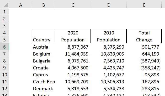
It is fairly common for users to format Excel reports with headers that are comprised of two or more rows for the header, rather than using a single cell with word wrap on. I’ve seen text files with similar issues as well. Consider the following example:

Getting this info into Power Query can sometimes be a challenge. I’m going to show you two ways to do it. The first way will be to do it manually mostly using the Power Query user interface. The second way will be a custom function that will do all of the work for you. For simplicity’s sake, I’ll use Power Query in Excel for this since my data is in Excel already, but the same logic would hold if you were importing the data into Power Bi. We do not want to consolidate the headers in Excel. You’ll just have to do it manually again the next time you get a file from someone. Remember - never pre-transform your data before you transform it in Power Query.

The Manual Method Using the Power Query Interface

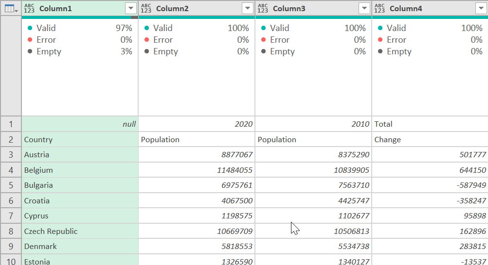
If you are using Excel, just put your cursor on the data somewhere and then the Data ribbon, select “From Sheet” if you are using Office 365. If you have an older version of Excel it may say From Table or Range. Make sure you uncheck “My table has headers” because it will only make the top row the header, and we don’t want that. Once you click OK, your data in Power Query window should look something like this:

If your Applied Steps to the right of the table have a Promoted First Row to Header and Change Type step, delete both of them. We just want everything to be in the data area, with columns named Column1, Column2, etc.

This example has two rows that need to be made the header. The process below though can handle any number of header rows. Just change the 2 to whatever it needs to be.

We need to break this table into two pieces - the first two rows, and everything but the first two rows. First, on the Power Query Home ribbon, select the Keep Rows button, Keep Top Rows, then type 2.

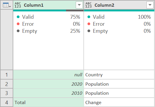
Now go to the Transform ribbon, and select Transpose. Your data should look like this:

So we’ve kept the top two rows, and rotated it 90 degrees so it is on its side. Now we just need to combine those two columns, transpose them again, then we need to go back and get the actual data. Here is how we will do that.

First, select both columns, then on the Transpose ribbon, select Merge Columns, and call it New Header. I chose a space as my separator.

Now to ensure there are no extra spaces, right-click on the new column and select the Transform, Trim command, and then again on the Transpose ribbon, the Transpose button. Now we have this:

We are almost there. We just need our data that we got rid of. It is still there in the Source line of our applied steps. This will require a little bit of modification of the M code in the formula bar.

To make this easier in a few minutes, you probably have a step called “Transposed Table1” in your applied steps. Rename that “NewHeader” with no spaces.

Next, right-click on NewHeader and select Insert Step After. In your formula bar it will say =NewHeader. Change that to read =Source. You’ll see we have our entire table back. Now, go to the Home ribbon, and select Remove Rows, Remove Top Rows, and type 2 - the same number of header rows our original Excel table had. Now we should just have our data with no headers at all.

I would rename this step “DataOnly” (again, no spaces) rather than the Removed Top Rows name. Here is where it gets interesting.

Go to the Home Ribbon and select Append Queries. Select the same query you are in. We are going to append this query to itself. It will show (Current) in the table name.

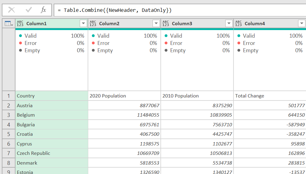
Right now our data is doubled up and we have no headers. Look at the formula bar. It should show this:

=Table.Combine({DataOnly, DataOnly})

Change the first DataOnly parameter to NewHeader. Now it looks more reasonable, and we have one header row at the top.

Now, on the Home ribbon, select Use First Row as Headers and change your data types. This is the final result:

At this point, you would probably get rid of the Total Change column, unpivot the Population columns to get it into a nice Fact table for Power BI’s data model, but that is another article. You can use this method for headers of any number of rows. I’ve seen some ERP systems export data with 2, 3, or 4 header rows. Just change the number of rows you keep or skip above to correspond to that.

The Custom Function Method

Now that you understand the logic, here is a custom function you can use to do all of that work for you. I am not going to walk through the code, but it is commented. I did it totally differently so it would be dynamic depending on how many header rows there were, handling different data types in the column headers, and how many columns were in the original data set. See below on how to put this in your model.

(OriginalTable as table, HeaderRows as number, optional Delimiter as text) =>
let
    DelimiterToUse = if Delimiter = null then " " else Delimiter,
    HeaderRowsOnly = Table.FirstN(OriginalTable, HeaderRows),
    /*  Convert the header rows to a list of lists. Each row is a full list
        with the number of items in the list being the original number of columns*/
    ConvertedToRows = Table.ToRows(OriginalTable),
    /* Counter used by List.TransformMany to iterate over the lists (row data) in the list. */
    ListCounter = {0..(HeaderRows - 1)},
    /*  for each list (row of headers) iterate through each one and
        convert everything to text. This can be important for Excel
        data where it is pulled in from an Excel Table and is kept
        as the Any data type. You cannot later combine numerical
        and text data using Text.Combine */
    Transformation = 
        List.TransformMany(
            ListCounter,
            each {ConvertedToRows{_}}, 
            (Counter, EachList) => List.Transform(EachList, Text.From)
        ),
    /*  Convert the list of lists (rows) to a list of lists (each column of headers is now in
        a list - so you'll have however many lists you originally had columns, and each list
        will have the same number of elements as the number of header rows you give it in the
        2nd parameter */
    ZipHeaders = List.Zip(Transformation),
    /*  Combine those lists back to a single value. Now there is just a list of the actual
        column header, combined as one value, using a space, or the chosen delimiter. */
    CombineHeaders = 
        List.Transform(
            ZipHeaders, 
            each Text.Trim(Text.Combine(_, DelimiterToUse))
        ),
    /*  Convert this list back to a single column table. */
    BackToTable = Table.FromList(CombineHeaders, Splitter.SplitByNothing(), null, null, ExtraValues.Error),
    /*  Transpose this table back to a single row. */
    TransposeToRow = Table.Transpose(BackToTable),
    /*  Append the original data from the source table to this. */
    NewTable = 
        Table.Combine(
            {
                TransposeToRow, 
                Table.Skip(OriginalTable, HeaderRows)
            }
        ),
    /*  Promote the new first row to the header. */
    PromoteHeaders = Table.PromoteHeaders(NewTable, [PromoteAllScalars=true])
in
    PromoteHeaders

To add this to Power Query do the following:

Create a new blank query. In Excel’s Power Query it is New Source, Other, Blank Query. In Power BI it is New Source, Blank Query.
Right-click on that new query and select Advanced Editor
Remove all of the code there so it is 100% empty.
Copy the code above - everything from the first row with “(OriginalTable” to the last row that says “PromoteHeaders” - and paste it into the Advanced Editor.
Press Done to save it
Rename it. It is probably called something useless like Query1. I usually use “fn” as a prefix to custom functions, and you want no spaces in it. So fnConsolidateHeaders as an example.

It should look like this in the Power Query window.

Now to use this. It is very simple. You want to start at the point your data in Power Query looks like the image above called “Original Table.” Way at the top. Yes, that is correct - it is immediately after getting your Excel grid of data into Power Query, and should be either the Source step or possibly the Navigation step depending on how your data is coming in. Please note: if you have aChanged Type or Promoted Headers step after the Source row, I recommend you delete them.

Now, right-click on that last step and select Insert Step After. Whatever is showing in the formula bar is the name of the table you need to modify. I will assume it is Source for this. In the formula bar, wrap that with this new function.

Here is the syntax of the function:

fnConsolidateHeaders(Table as table, Number of Header Rows as number, optional Delimiter as text)

Table - this is the table name - so Source, or whatever the name of the immediate step above is. Again, right-click that step and select insert Step After and the table name will be there in the formula bar for you.
Number of Header Rows - type in an integer of how many header rows there are in the data. 2, 3, whatever.
optional Delimiter - this is what you want to be between the header rows when they are concatenated. This is optional. The formula will use a space if you put nothing there, but you can use any character(s) you want. You can even have no delimiter if you type two quotes with nothing in between - ““. This is a text field, so you must enclose your delimiter in quotes.

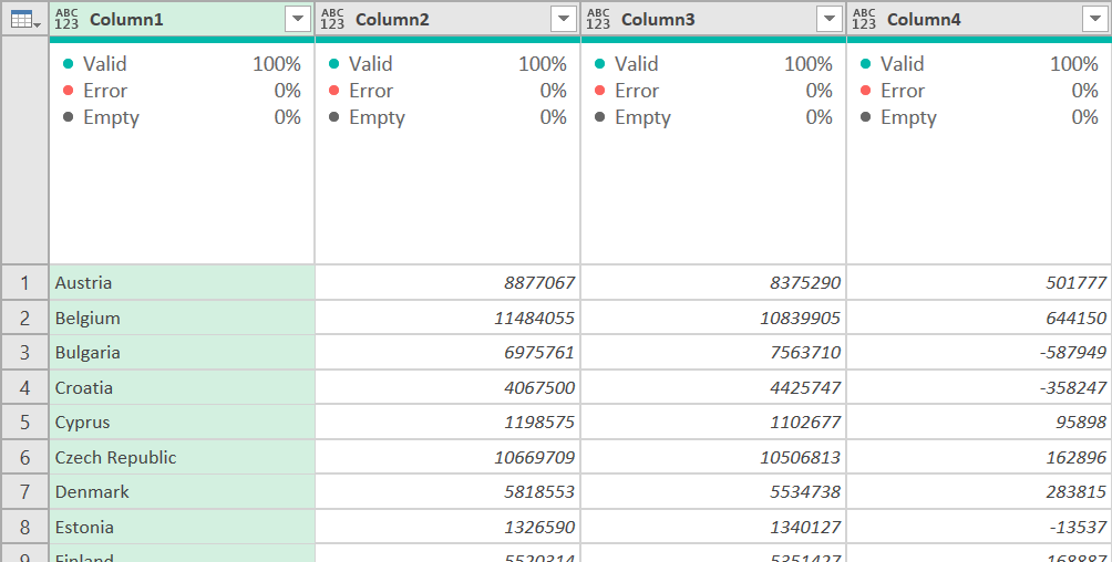
That’s it. It should return this:

Now you have one final step. Change all of the columns to the correct data types.

Hopefully this will help you when dealing with Excel reports, or even some CSV/Text files, where there are multiple rows used for the header.
Finally - here is the Excel file with the sample data and full code for doing this manually or with the custom function.

Ed Hansberry's Power BI and Excel Blog

Working With Multiple Row Headers From Excel in Power Query

The Manual Method Using the Power Query Interface

The Custom Function Method

ehansalytics

Business Analytics